Diffusion Models for Simulated-to-Real US Image Conversion
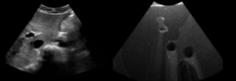
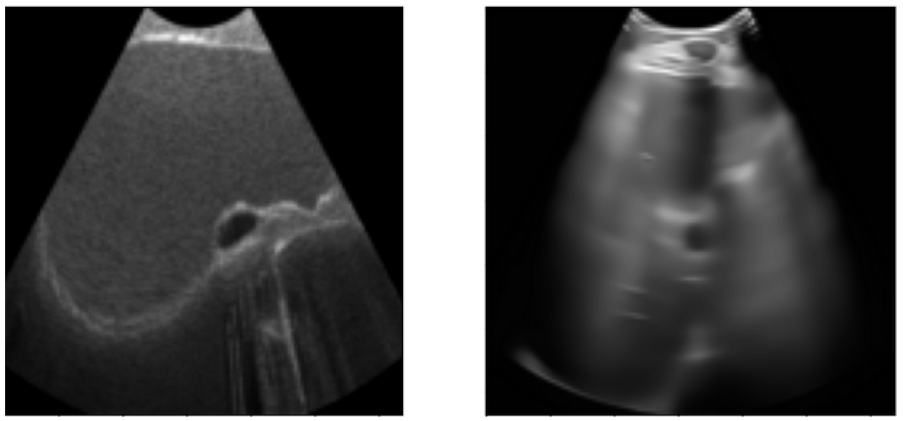
Ultrasound (US) images are inconsistent compared to other image modalities. They could vary depending on the operator, machine or even the pressure applied. Hence it is difficult to gather large consistent datasets for computer vision applications. One way to quickly generate consistent US images is to simulate them from 3D CT scans. But the simulated images do not look realistic enough and lack the fine grain details such as specular reflections or noise.
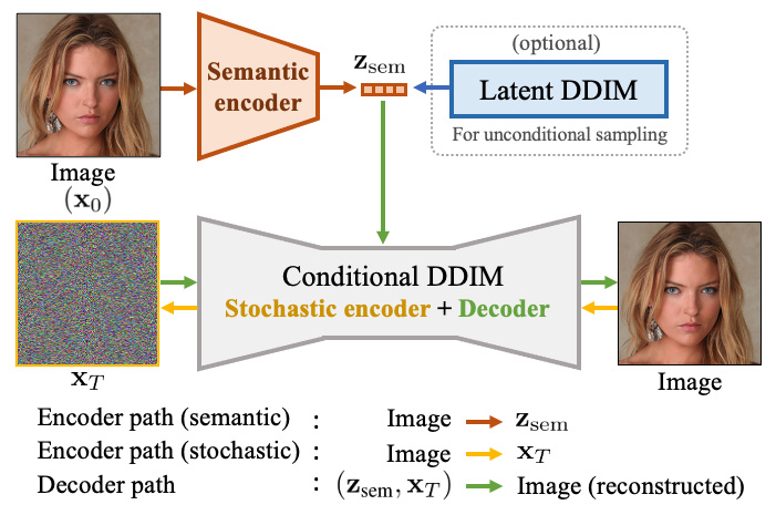
Diffusion Autoencoder has a familiar autoencoder architecture that uses a semantic encoder to capture high level semantic information about the input and encode it into a vector. The decoder, in contrast to a typical autoencoder, is a denoising diffusion implicit model (DDIM). DDIM has two main tasks; first it stochastically encodes the input image into a stochastic subcode (XT). Secondly, given the stochastic subcode image and its vector representation it decodes the image back into the original input. An overview of the models architecture can be seen in the figure below. For the scope of this project the latent DDIM (blue in figure) can be ignored.
Furthermore, this model allows for the manipulation of the semantic and stochastic representations of the input to change the different attributes of the output image. This ability of the model was used in two different ways in this work for simulated to real ultrasound translation.
The network was trained using simulated and real US dataset of 12000 images. The simulated images were generated using the ImFusion software from CT scans. EMA (exponential moving average) was used to update the parameters of the model.
In order to evaluate the training performance of the network the FID score was calculated based on 1200 sample images. Because this number is lower than the usual 50000 images used to calculate FID scores and because FID is not generally made for medical images, the features from the second max pooling layer of the InceptionNet were used (instead of the last). Different noise schedulers were tested and the best performing model used cosine scheduling with an FID score of 4.5.
Simulated to Real US translation
There are two main methods that this project focused on to move between simulated and real domains. The first method was interpolation between the vector representations of the images. The intuition behind this method is that the semantic space is meaningful and moving linearly between two points should result in new meaningful images that gradually change from the first image to the second one.

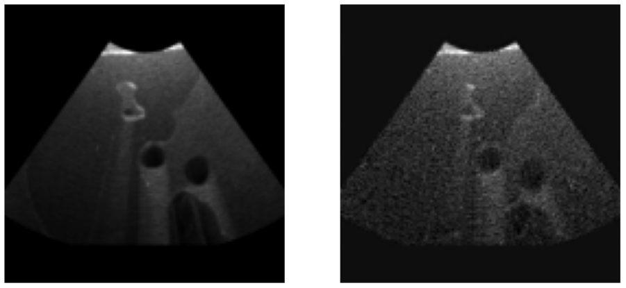
The second method is to manipulate the vector representation of the images based on a linear classifier. A linear classifier is trained to classify between simulated and real US images. The weights of this classifier is multiplied with some factor and added or subtracted from the semantic vector of the image. The modified vector is used as a condition to guide the diffusion process. Two classifiers were trained for this method, one using binary cross entropy (BCE) loss and another one with mean squared error (MSE) loss. You can see the results of the manipulated images below.
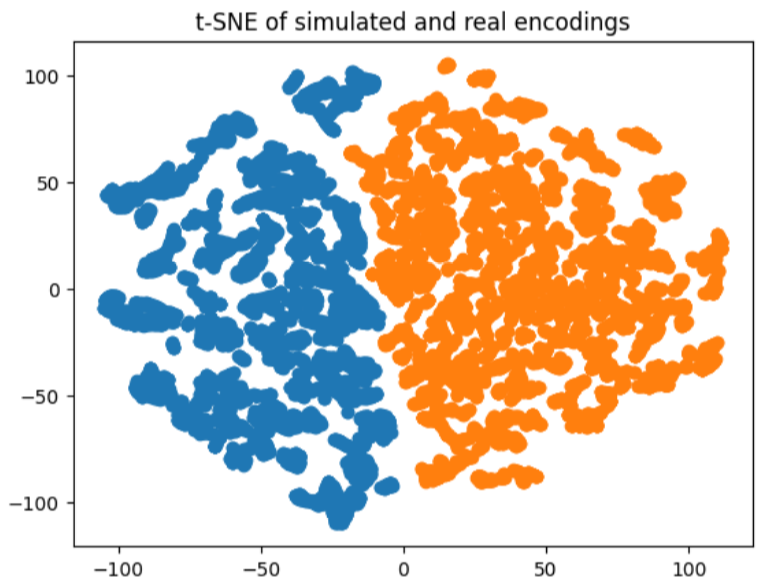
Overall, this project was very fun to work on. Unfortunately, due to limited amount of data it was not possible to reliably generate realistic looking US images. The differences between the simulated and real US images are too much and the network is easily able to differentiate between them. This becomes more clear when looking at the t-SNE of the simulated and real vector representations.